A Predicting Wave Heights from Floating Buoy Data

Tyler Kim

Final project for 6.7960, MIT

Motivation

Approximately 71% of the Earth's surface is covered by water. Prior to the 15th century, the ocean posed a barrier between the various socieities of the world. Humanity's ability to traverse the ocean was the tipping point of recent history, as disparate geographies were now acessible to each other. Trade of spices, cultures, and ideas between foreign lands has ushered in an era of globalization that shapes every aspect of our lives today.

The ocean still has potential to continue revolutionizing life on Earth. In the face of growing climate crises, wave energy could serve as a new source of renewable energy. Wave energy is much more reliable, and an order of magnitude more powerful than wind energy, according to [1]. One vital characteristic of wave energy is wave height.

Beyond renewable energy, wave height plays an important role in commercial shipping, for both boat activity [2] as well as port operations [3]. Additionally, water sports like surfing rely on accurate predictions of wave heights. The global market for surfing is estimated to reach $5.5 billion by 2030 [4], and companies like Surfline play a crucial role in the industry by providing surf forecasts.

Given the importance of wave heights, many approaches to wave forecasting have been devised. WAVEWATCHCIII (Tolman, 1991), a physically-based engineering model, is still widely used in practice today. However, WAVEWATCHCIII is numerical solver [5], which are computationally intensive and make assumptions of natural phenomena.

Recently, deep learning methods have been proposed to perform wave forecasting, including LSTM [9] and transformer based approaches [8]. However, the current literature considers the forecasting task for a single buoy, given the previous data from that buoy. Since wave energy travels throughout the ocean, it is reasonable to assume that past wave data from nearby locations will be relevant to the prediction task. This project explores the impact of providing the model with data from nearby buoys for the prediction task of wave height.

Luckily for researchers, the National Oceanic and Atmospheric Administration, a division of the US Department of commerce, collects data on ocean condititions from buoys stationed around the world. Using this data, I train a transformer-based neural network to predict wave heights. I modify the standard transformer architecture by utilizing custom dataset generation logic, which allows for the inclusion of wave data from nearby, offshore buoys to provide additional context to the prediction task at nearshore locations.

Data

The dataset is collected from the National Oceanic and Atmospheric Administration (NOAA). The NOAA stations buoys around the world that collect data on wave factors. A full description of the data can be found at the data description here.

Data Preprocessing

The data is recorded at the minute level for the year 2023. To reduce the complexity of the dataset, and to avoid exceedingly large context windows, I convert the data to hourly samples by taking the last record for each hour. The data also contains missing values, which are encoded as "999" or some value with 9's in each digit.

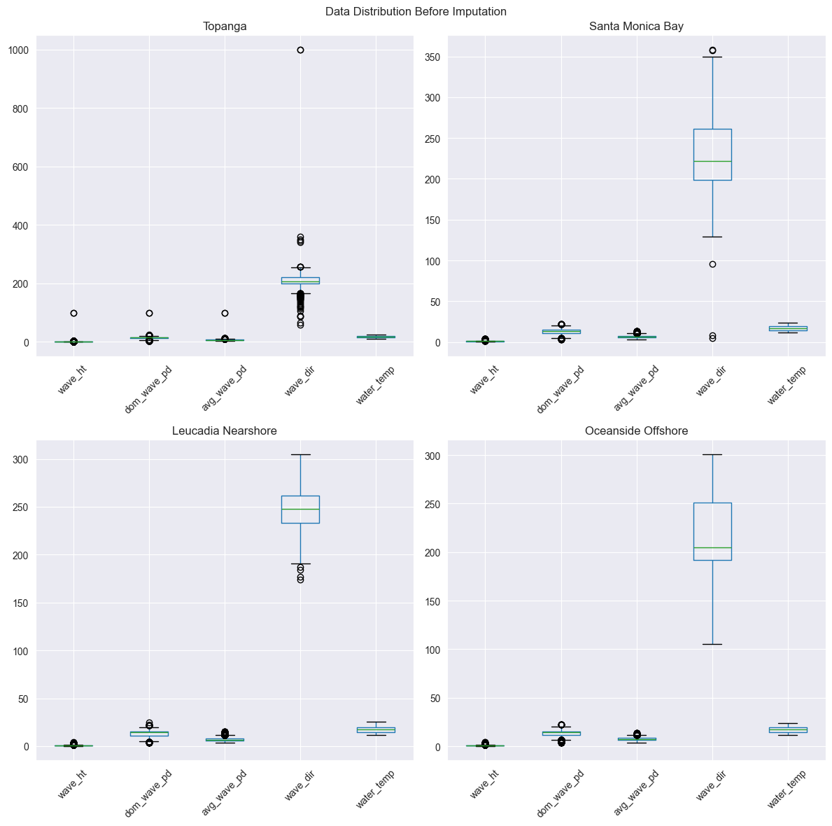
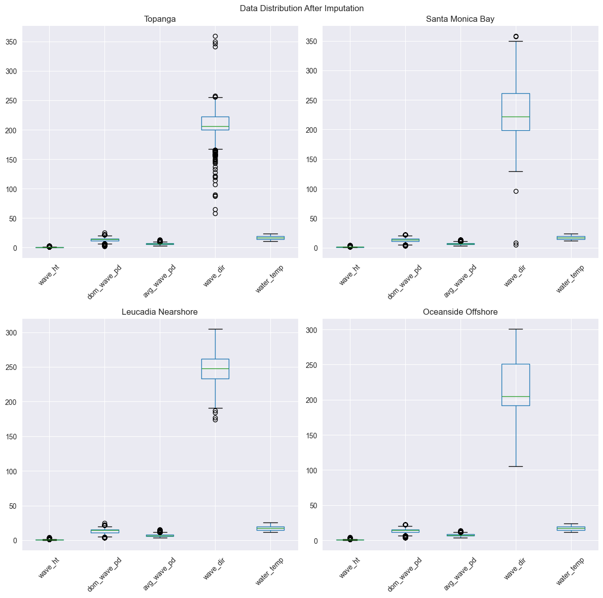
After dropping the missing values, we are left with:

• Wave Height
• Dominant Wave Period
• Average Wave Period
• Wave Direction
• Water Temperature

Within the columns we keep, there are still additional missing values that are randomly dispersed throughout the dataset. These missing values are also encoded as "999" or some value with 9's in each digit. These differences can actually be observed, and boxplots of the data distribution before imputation and after imputation are shown in the appendix. We can see that the Topanga buoy has outlier values of 9999 for wave direction. Additionally, while it is harder to see due to the scale, there are also outliers for wave height, dominant wave period, and average wave period. While values of 99 are not technically impossible, the fact that these outliers occur at exact values of 99 indicates that they are likely truly missing. These random missing values are imputated according to the mean of a rolling average from a window of 10 hours before and after the missing value.

Data Exploration

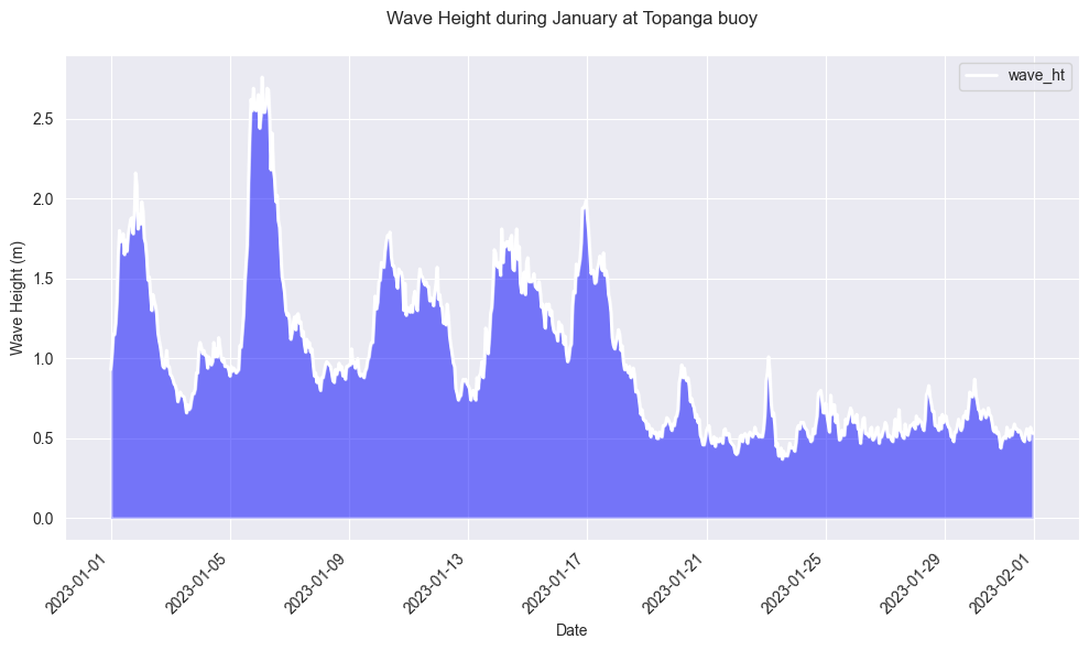
For the rest of the analysis, we are interested in predicting wave height. To understand the form of the target variable, a plot of wave height data from the Topanga buoy in the month of January 2023 is shown below:



There is a fair amount of periodicity, as well as some variability with seasons, such as a large spike in wave height at the start of January. This tracks relatively well with intuition, as swell waves are generated by storms throughout the Pacific Ocean during the winter months. [7]

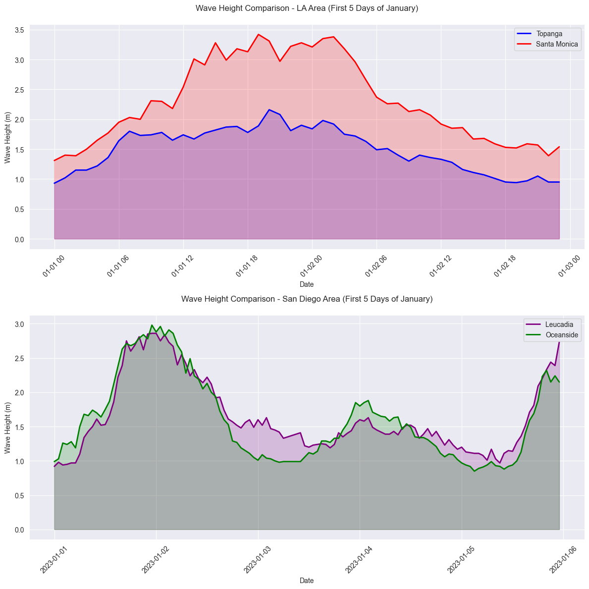
In our analysis, we consider two offshore-nearshore buoy pairs --- Leucadia and Oceanside, and Topanga and Santa Monica. To see the comparisons between the heights of waves at the two locations, a 4 day selection is plotted below (note that Santa Monica/Topanga are in LA, and Leucadia/Oceanside are in San Diego).

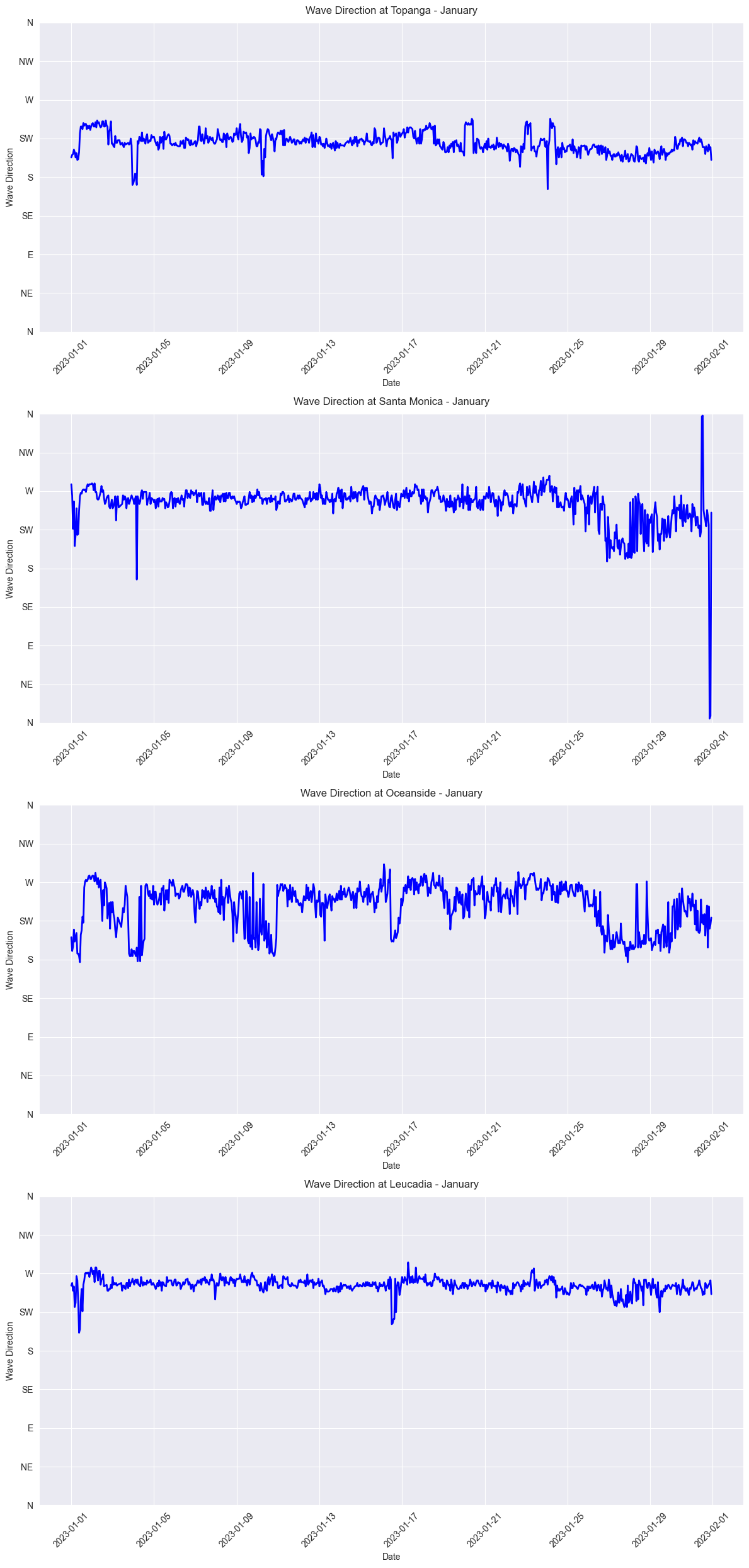
To better understand other columns, like the wave direction, a plot is included in the appendix. With an understanding of our dataset, we can begin to discss the details of the wave height prediction model.

Architecture

The proposed algorithm begins with the dataset generator. Prior work on wave height prediction considers the canonical forecasting task --- given a stream of consecutive data realizations indexed by time, use previous realizations to predict future values [6]. Formally, they seek a function $f^*(\cdot)$ that produces predictions $\hat{Y^*}$ given a time-indexed sequence of data $X_n$. $$f^*(X_t | X_{t-w}, X_{t-w+1}, ... X_{t-1}) = \hat{Y^*_t}$$ for context window size $w$. The function is optimal in the sense that it produces predictions with minimal loss/error: $$f^* = \arg \min_f \mathbb{L}(f(x), y)$$ where $\mathbb{L}$ is a loss function.

However, due to the nature of ocean currents, we have additional information that would be relevant to the prediction task --- wave data from nearby buoys. The prediction task would then become $$f^*(X_t | \{X_{t-w}, X_{t-w+1}, ... X_{t-1}\} \cup \{Z_{t-k-w+1}, Z_{t-k-w+2}, ... Z_{t-k}\}) = \hat{Y^*_t}$$ with $Z$ being the data from the nearby buoy, time lag $k$, and context window size $w$. Theoretically, as long as Z is not excessively noisy, the additional information should improve the model's predictive power.

The assumption that Z is not noisy is reasonable to make. Wave energy travels throughout the ocean, and wave energies propagate in predictable ways. For example, the California Current travels southward along the West Coast of the United States from British Columbia, Canada, to the southern tip of California.

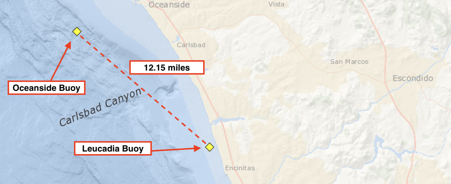
In our dataset, we utilize a more readily observable oceanic phenomenon --- the flow of water towards the shore, creating the waves that make California's beaches famous. The locations of two of the buoys in our dataset are shown below:



The dataset generator takes in data from two buoys --- one offshore, and one nearshore. The generator produces $(\text{nearshore data}, \text{offshore data}, \text{target})$ triplets. Becuase the number of FLOPs grows quadratically with the size of the context window in the attention mechanism, we restrict the "context" (number of trailing timesteps before target) to be 24 --- since our data is sampled every hour, the model has access to the previous 24 hours worth of data when generating a prediction of wave height.

I also include an additional parameter k, to control the time lag between the offshore and nearshore buoys. To understand the function of k, consider an offshore buoy that is very far from the nearshore. The slice of the offshore buoy's data should be adjusted to account for the time that it takes for the wave energy to travel from the offshore buoy to the nearshore buoy. Formally, we provide training samples to the model in the form of $$(\text{nearshore data}[t-24:t-1], \text{offshore data}[t-k-24:t-k-1], \text{target}[t])$$

From this definition, we can see that increasing k, the time lag, will result in the model being trained on older slices of offshore buoy data. In our hypothetical example above, higher k would allow the model to access offshore buoy data that is relevant to the prediction task.

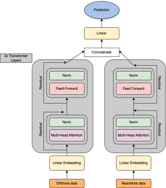
The model itself consists of an initial linear embedding layer, two multi-head attention layers, and a linear output layer. Both the nearshore and offshore data are passed through a separate transformer block, mean pooled, and concatenated. The concatenated data is passed through a final linear layer to produce the prediction. I train the model for 15 epochs, batch size 128, and learning rate 0.001. A diagram of the architecture is shown below



The introduction of the new parameter k creates a natural question --- how should we choose the value of k? In this project, I take a simple approach and performs a search over a few reasonable values of k, and choose the model with the best performing k. Values of k come from a set of candidate values $[1, 12, 24, 48, 168]$. The construction of our training data means that for $k = 48$, the prediction task for time $t$ will utilize offshore buoy data from 2 days prior, with a 24-hour context window.

I use the mean squared error (MSE) as the loss function, and to judge the marginal value of providing data from offshore buoys, I compare against a model in the canonical forecasting task: predicting the value of wave height at the nearshore buoy at time $t$ given data from the buoy at times $[t-24, t-23, ... t-1]$.

Results

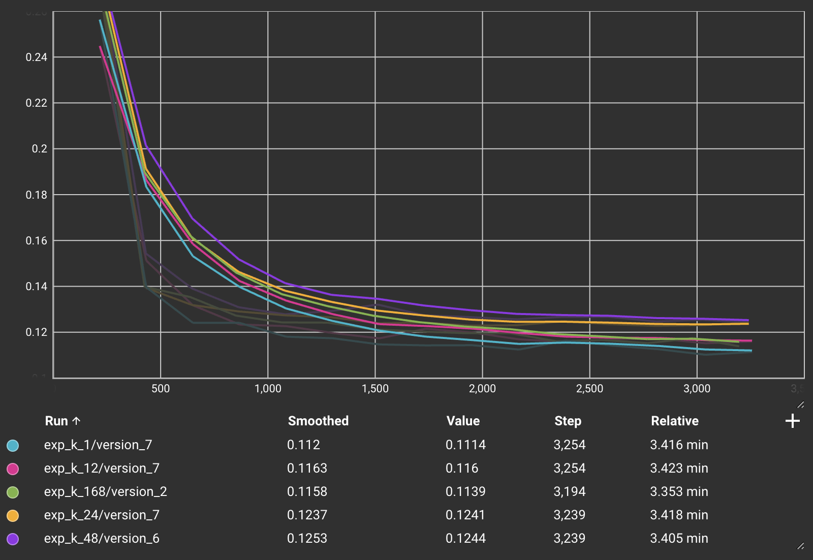
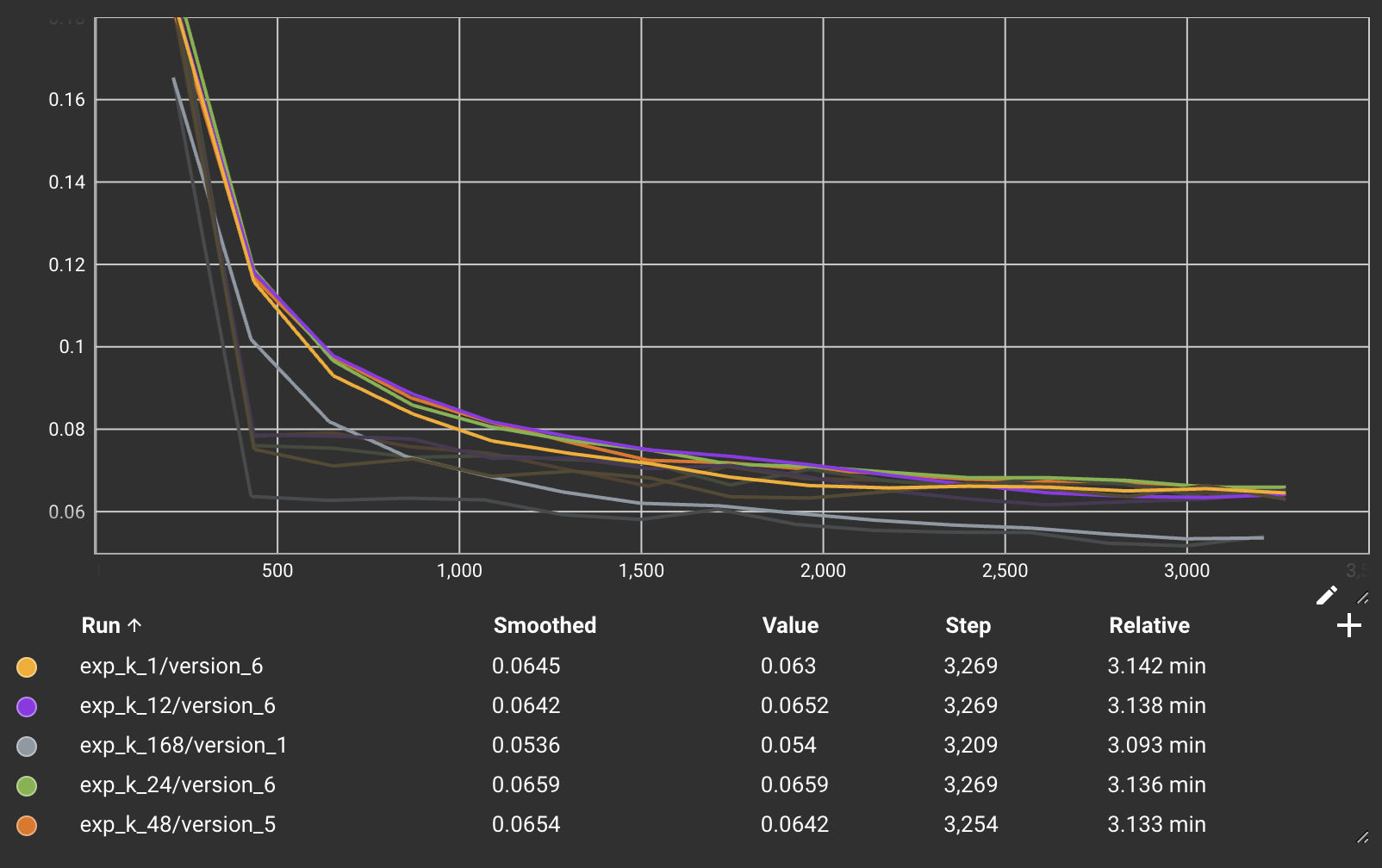
Results of training for the LA buoys (Santa Monica, Topanga) and SD buoys (Leucadia, Oceanside) are shown below:

Training Loss Curve for Leucadia (y-axis is MSE loss, x-axis is step)

Training Loss Curve for Topanga (y-axis is MSE loss, x-axis is step)

For the Topanga buoy, the model with $k=168$ (7 days) achieves the lowest training loss at 0.053. When tested on a validation set, the model with $k=12$ achieves the lowest training loss, with 0.054. For the Leucadia buoy, the model with $k=1$ achieves both the lowest training loss and validation loss at 0.111 and 0.114, respectively.

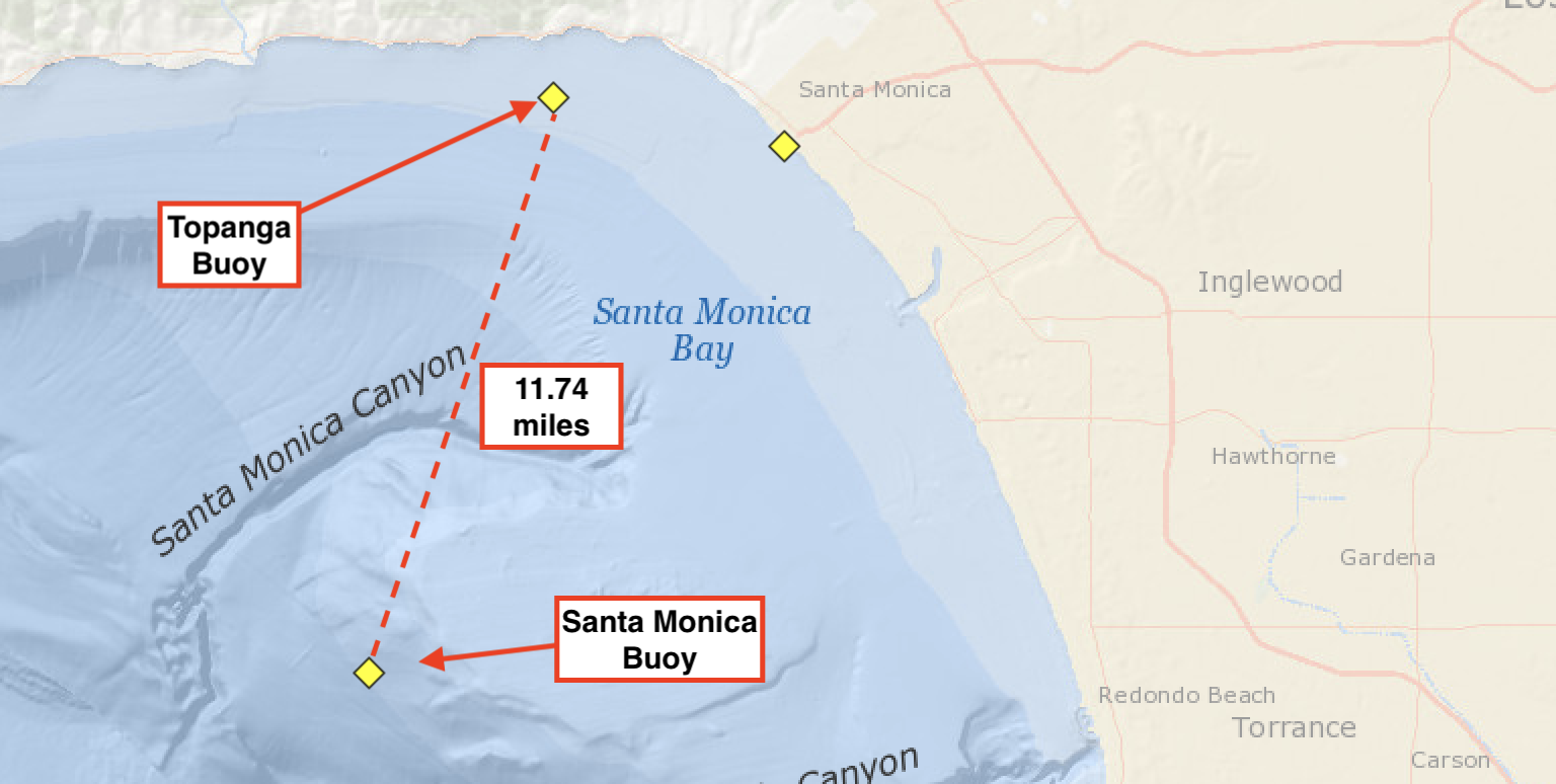
The results indicate that the Topanga buoy depends differently on the offshore buoy data than the Leucadia buoy. Interestingly, despite the Topanga buoy being closer to its offshore buoy (11.74 miles vs. 12.15 miles), the optimal time lag $k=12$ hours for Topanga, while it's only 1 hour for Leucadia. What is the cause of this discrepancy? Looking at the buoy locations plotted below, we can see that the orientation of the nearshore buoys relative to the offshore buoys are different.



Recalling the southward flow of the California Current, we can see that the Leucadia buoy is in the direct path of ocean flows, whereas the Topanga buoy is not --- in fact, the Topanga buoy is above the Santa Monica Bay buoy. However, the ocean flows through Santa Monica Bay can still propagate towards the Topanga buoy, due to the formation of eddies, which can be caused by wind effects, instabilities in ocean currents, and differences in water temperatures and densities. Eddies, along with coastal topographies like the Palos Verdes Pensinsula create the phenomenon known as the Southern California Counter Current --- a northward flow that opposes the direction of the California Current. Naturally, this indirect path means that the wave energies from the Santa Monica Bay will take longer to reach the Topanga buoy, as reflected by larger time lags $k$. Intererstingly, our model has learned to pick up on this relationship through the flexible context window for offshore data. This indicates that even buoys which lie outside the typical flow of current could be helpful in predicting wave heights.

The key question is whether using offshore buoy data actually improves the model's performance. Below, we compare the model's validation loss when trained on both offshore and nearshore buoy data versus just nearshore buoy data:

Location	Data Used	Validation Loss (MSE)
Leucadia	Nearshore + Offshore	0.11
	Nearshore Only	0.12
Topanga	Nearshore + Offshore	0.054
	Nearshore Only	0.06

The results show a slight improvement in MSE by adding offshore data. One interesting extension to consider would be to add more buoys to the dataset, and see if model prediction is benefitted by context from other locations.

Conclusion

In this analysis, we explored the potential of using offshore buoy data to improve wave height predictions at nearshore locations. Our findings suggest that incorporating offshore data leads to slight improvements in validation loss, or equivalently, prediction accuracy in terms of MSE. Promisingly, there is indication that the model gains predictive capacity depending on the relevance of the time-slice of data from the offshore buoy that we provide. The notions of "relevance" corresponds to what we might believe to be intuitively true, as discussed when considering the much larger time lag for the Topanga buoy due to counter currents.

While the improvements in prediction accuracy are relatively small, the approach lends itself well to extension based on additional data from neighboring buoys. The NOAA data is quite comprehensive, and many buoys have nearby buoys in a multitude of directions. Additionally, an approach to making the time-lag parameter k optimizable was discussed.

Appendix

1. Results of data before & after imputation

2. Wave directions during the month of January